We've begun publishing the Exon CLI to the AWS Public ECR. This means you can pull and run the Exon CLI using Docker, and use it interactively or in scripts and workflows, like Nextflow which we'll see in a second.

For example, say I was in a directory with a single FASTA file, test.fasta. I could "drop" into the Exon CLI using the following command:

docker run -it -v $(pwd):/data where-true-tech/exon-cli:latest

Which would start the Exon CLI and drop me into a shell. And from there, I could query the data.

❯ SELECT * FROM fasta_scan('/data/test.fasta');
# +----+--------------+----------+
# | id | description  | sequence |
# +----+--------------+----------+
# | a  | description  | ATCG     |
# | b  | description2 | ATCG     |
# +----+--------------+----------+
# 2 rows in set. Query took 0.026 seconds.

While we plan on releasing native binaries for the Exon CLI, with Docker, you can easily use the CLI in your workflows and scripts.

Nextflow Example​

Nextflow is one of the most popular workflow managers for bioinformatics. It's a great tool for building reproducible workflows, and it's easy to use the Exon CLI in Nextflow workflows.

For example, if I wanted to copy a FASTA file generated earlier in the workflow, into Parquet for warehouse storage, I could use the -c (command) flag to execute a COPY query in the Exon CLI. This would look something like the following:

As a minimal example, we can round-trip a FASTA file from S3 to Parquet using the Exon CLI and Nextflow. In reality, whatever relevant domain task would generate the FASTA, and then we could use the Exon CLI to copy it into Parquet.

// main.nf
process copyFastaLocally {
    output:
    path 'test.fasta'

    script:
    """
    aws s3 cp s3://wtt-01-dist-prd/tmp/test.fasta .
    """
}

process exportToParquet {
    container 'public.ecr.aws/where-true-tech/exon-cli'

    input:
    path input_fasta

    script:
    """
    exon-cli -c "COPY (SELECT * FROM fasta_scan('$input_fasta')) TO 's3://wtt-01-dist-prd/tmp/test2.parquet' (FORMAT PARQUET)";
    """
}

workflow {
    main:
    copyFastaLocally()
    exportToParquet(copyFastaLocally.out)
}

In order to use Docker and have it access AWS, you'll need to make sure your nextflow.config is configured for them. For this example, the following configuration would be sufficient:

// nextflow.config
docker {
    enabled = true
    envWhitelist = 'AWS_ACCESS_KEY_ID,AWS_SECRET_ACCESS_KEY'
}

Conclusion​

We hope you find the Exon CLI tool useful to support you taking advantage of modern data warehousing and analytics tools in your bioinformatics workflows. If you'd to learn more about what options are available to you, please check out the CLI documentation. Also, if you need more flexibility than the CLI provides, you can always use the BioBear with Python.

If you have any questions or feedback, please reach out to us on at wheretrue.com/contact or on Twitter.

This post will walk through some of the recent updates to Exon, and show how they can be used with BioBear and/or ExonR.

These updates include:

• Addition of several table functions to scan various bioinformatic files and query some indexed files. Using these table functions requires less boilerplate SQL code, so are a nice quality of life improvement.
• Exon has gain the ability to do index seeks on GFF files for region queries. Now users can access specific regions across large annotations sets without resorting to costly sequential scans.
• Flow Cytometry Standard (FCS) files are now supported, and can help scientists go very quickly from the FCS binary format to a DataFrame for analysis.
• Various optimizations led to performance improvements for bgzipped files.
• New utility table types where added to align more simply to file extensions: FNA (.fna), FAA (.faa), FQ (.fq).

Table of Contents

• Table Functions
• Scanning and Querying
  • Example Scanning Function
  • Example Query Function
• Indexed GFF Files
• Flow Cytometry Standard (FCS) Files
• Faster bgzip Reading
• New Utility File Types
• Conclusion

Table Functions​

The addition of table functions is mostly a quality of life improvement, but it's good to live good, so to speak. A table function returns a table that is incorporated into the larger query plan. For example in

SELECT COUNT(*) FROM gff_scan('gff/test.gff.gz');

gff_scan creates a table which is then incorporated into the overall query to count the contents of that file. This is the same thing as doing:

CREATE EXTERNAL TABLE gff_file
STORED AS GFF
COMPRESSION TYPE GZIP
LOCATION 'gff/test.gff.gz';

SELECT COUNT(*) FROM gff_file;

As you can see, it's considerably less typing. Or, if we were to use BioBear, we can see it's ease:

import biobear as bb

sess = bb.connect()
df = sess.sql("SELECT * FROM gff_scan('gff/test.gff.gz')").to_polars()
print(df.head())

There's the obvious downside in that the table function can't be reused like the table, which is not in the database's catalog. However, given these are backed by an external file, which won't change, it's often moot.

Scanning and Querying​

As of this release, there are two types of table functions available: scanning, for bulk scanning of all underlying records, and querying, for specific region access for indexed files.

Please see the table function docs, for what's specific available, but generally all current files have scan support, and indexed files are VCF, SAM, and GFF.

Example Scanning Function​

Scanning functions take a couple of options. First, they all require the location of the table. This can be a single file or a folder. Second, if applicable, they can take the compression of the underlying file. The table function will also try to use infer the compression type, but this only works for single files. If you pass a folder/prefix, you must pass a compression type unless the files are actually uncompressed.

So, we already saw one example, but we can also can other file types and potentially include them in larger queries. For example,

SELECT *
FROM fasta_scan('fasta/test.fasta') AS f
    JOIN gff_scan('gff/test.gff.gz') AS g
        ON f.id = g.seqname;

Again, see the table function docs for the list of available functions, and more examples.

Example Query Function​

Querying indexed files can save a lot of time because only the bytes that belong to the query region are included. The newly adding bam_indexed_scan, vcf_indexed_scan, and gff_indexed_scan, allow querying those respective files.

With BioBear, we an easily write a script which can search regions and save the results as parquet.

def query(path: str, region: str):
    sess = bb.connect()
    df = sess.sql(f"SELECT * FROM vcf_indexed_scan('{path}', '{region}')").to_polars()
    df.write_parquet(f"{region}.parquet")

if __name__ == "__main__":
    query("vcf/index.vcf.gz", "1")

Indexed GFF Files​

As mentioned, Exon can now do index seeks on GFF files to markedly reduce query times when a specific sequence or region is needed.

This access pattern comes up often. For example, in metagenomics to get the neighboring annotations for an enzyme of interest. Or in human health, to query regions near some pathogenic variant.

Similar to SAM and VCF index support in Exon, there are two ways to run queries. First, the gff_indexed_scan, like so:

SELECT COUNT(*)
FROM gff_indexed_scan('gff-index/gencode.v38.polyAs.gff.gz', 'chr1:1000000-2000000')

You must have an index file associated with the gff file at gff-index/gencode.v38.polyAs.gff.gz.tbi.

Similarly, you can make a table, then query it to your heart's content.

CREATE EXTERNAL TABLE indexed_gff
STORED AS INDEXED_GFF
COMPRESSION TYPE GZIP
LOCATION 'gff-index/gencode.v38.polyAs.gff.gz';

And to query:

SELECT COUNT(*)
FROM indexed_gff
WHERE gff_region_filter('chr1:1000000-2000000', seqname) = TRUE;

Flow Cytometry Standard (FCS) Files​

FCS files are the output from flow cytometry experiments. They are binary files, and can be quite large. Exon can now can incorporate them in queries, and used with BioBear and ExonR by extension. For example, to scan a file with BioBear and load it into a DataFrame:

import biobear as bb

sess = bb.connect()
df = sess.sql("SELECT * FROM fcs_scan('fcs/Guava Muse.fcs')").to_polars()
print(df.head())

And that will output a table that looks like:

As a next step, you could select specific columns (via the SELECT clause) or rows (via the WHERE clause) to further refine the query, and then pass the results to a plotting library or other analysis tool.

Faster bgzip Reading​

Reading some compressed formats as gotten faster due to build improvements. For example, comparing The last version to this one when reading a larger VCF file, we see that the new version is about 1.5x faster than the last.

hyperfine './exon-benchmarks-v0.5.0 vcf-query -p WGS.vcf.gz -r chr1:10000-10000000' './exon-benchmarks-latest vcf-query -p WGS.vcf.gz -r chr1:10000-10000000'
Benchmark 1: ./exon-benchmarks-v0.5.0 vcf-query -p WGS.vcf.gz -r chr1:10000-10000000
  Time (mean ± σ):      1.430 s ±  0.055 s    [User: 5.784 s, System: 0.625 s]
  Range (min … max):    1.361 s …  1.553 s    10 runs

Benchmark 2: ./exon-benchmarks-latest vcf-query -p WGS.vcf.gz -r chr1:10000-10000000
  Time (mean ± σ):     952.6 ms ±  69.7 ms    [User: 3319.4 ms, System: 513.8 ms]
  Range (min … max):   895.1 ms … 1117.4 ms    10 runs

Summary
  './exon-benchmarks-latest vcf-query -p WGS.vcf.gz -r chr1:10000-10000000' ran
    1.50 ± 0.12 times faster than './exon-benchmarks-v0.5.0 vcf-query -p WGS.vcf.gz -r chr1:10000-10000000'

New Utility File Types​

Because sequence files often have different extensions, e.g. .faa for a FASTA file consisting of Amino Acids, it can be annoying to manage that difference via the extension vs having a specific table type.

So now that are a few new table types to simplify things:

Conclusion​

We hope these updates make Exon, BioBear and ExonR, more useful for your bioinformatics needs. If you have any questions, please feel free to reach out.

In an effort to make it easier for our users to connect with the existing tools in their stack, we're excited to announce that Exome now supports communicating over the Postgres wire protocol. What this means is that users can use psql in the console or psycopg2 to connect to Exome and query their data.

To be clear, Exome does not yet support the pg_catalog system catalog, meaning that many BI dashboard and ETL tools will not work with Exome yet. However, we're working on adding support for pg_catalog and hope to have it available soon.

Connecting to Exome with psql​

Assuming you've made an Exome user, you can connect the example catalog in Exome with psql using the following command:

psql -W -H pg.exome.wheretrue.com -U test@mail.com -d public.example_library.example_catalog

If that all goes well, you'll be prompted for your password and then connected to the Exome catalog. You can then run queries as you would with any other Postgres database.

$ psql -W -H pg.exome.wheretrue.com -U test@mail.com -d public.example_library.example_catalog
psql (14.9 (Homebrew), server 0.1.0)
SSL connection (protocol: TLSv1.3, cipher: TLS_AES_256_GCM_SHA384, bits: 256, compression: off)
Type "help" for help.

public.example_library.example_catalog=>

We can then run queries as we would with any other Postgres database.

public.example_library.example_catalog=> SELECT COUNT(*) FROM example_catalog.example_schema.fasta_table;
 cnt
-----
 500
(1 row)

public.example_library.example_catalog=> SELECT id, description FROM example_catalog.example_schema.fasta_table LIMIT 5;
         id          |                                                description
---------------------+-----------------------------------------------------------------------------------------------------------
 UniRef50_A0A5A9P0L4 | peptidylprolyl isomerase n=1 Tax=Triplophysa tibetana TaxID=1572043 RepID=A0A5A9P0L4_9TELE
 UniRef50_A0A410P257 | Glycogen synthase n=2 Tax=Candidatus Velamenicoccus archaeovorus TaxID=1930593 RepID=A0A410P257_9BACT
 UniRef50_A0A8J3NBY6 | Gln_amidase domain-containing protein n=2 Tax=Actinocatenispora rupis TaxID=519421 RepID=A0A8J3NBY6_9ACTN
 UniRef50_Q8WZ42     | Titin n=3053 Tax=cellular organisms TaxID=131567 RepID=TITIN_HUMAN
 UniRef50_A0A401TRQ8 | Ig-like domain-containing protein (Fragment) n=2 Tax=Chiloscyllium TaxID=34767 RepID=A0A401TRQ8_CHIPU

Connect to Exome with psycopg2​

psycopg2 is a popular Python library for connecting to Postgres databases. It's used by many Python libraries and frameworks, including Django and SQLAlchemy. To connect to Exome with psycopg2, you'll need to install the psycopg2 package in your python environment.

pip install psycopg2

Once you've installed psycopg2, you can connect to Exome with the following code:

import psycopg2

conn = psycopg2.connect(
    host="pg.exome.wheretrue.com",
    port=5432,
    user="user@example.com",
    password="RainbowsAndUnicorns",
    dbname="public.example_library.example_catalog",
)

conn.autocommit = True

cur = conn.cursor()
cur.execute("SELECT COUNT(*) cnt FROM example_catalog.example_schema.fasta_table;")
print(cur.fetchone())

If that all goes well, you should see the following output:

(500,)

What's Next?​

We're working on adding support for pg_catalog and hope to have it available soon. If you have any questions or feedback, please reach out to us at support@wheretrue.com.

Signup for Exome to try it for yourself.

In addition to launching the public preview of Exome last week, we've also made some updates to Exon.

First, Exon now supports Hive style partitions. This means you can augment your table definitions with partition information. This is useful because:

1. It allows you to augment your file schemas with additional metadata. For example, the experiment date, or the sample type.
2. It allows you to query subsets of your data without having to scan the entire table. For example, you can query only the data from a specific sample.

Second, ExonR has been updated to support a SQL session allowing you to create and query tables directly from R, rather than just scan entire files.

Finally, as more of an administrative note, we've added a GitHub Sponsors page. If you find our open source software useful, please consider sponsoring us. Thanks!

Table Partitions​

Table partitions are encoded in the file path when you store the data and additionally in the table definition.

For example, say you had a bunch of S3 objects at:

s3://bucket/fasta_table/sample=sampleA/file1.fasta
s3://bucket/fasta_table/sample=sampleA/file2.fasta
s3://bucket/fasta_table/sample=sampleA/file3.fasta
s3://bucket/fasta_table/sample=sampleB/file4.fasta

You could create a table definition like:

CREATE EXTERNAL TABLE fasta_table
STORED AS FASTA
PARTITIONED BY (sample)
LOCATION 's3://bucket/fasta_table'

Then you could query the data like:

SELECT *
FROM fasta_table
WHERE sample = 'sampleA'

And what happens is super useful, Exon will subset the files it scans based on the predicated and augment the FASTA table with the sample column.

So you end up with something like:

Moreover, this makes it straight forward to join with other data. For example, if you had a table of sample metadata:

CREATE EXTERNAL TABLE sample_metadata
STORED AS PARQUET
LOCATION 's3://bucket/sample_metadata/'

You could join the two tables like:

SELECT *
FROM fasta_table
JOIN sample_metadata
ON fasta_table.sample = sample_metadata.sample

Thus simplifying your analysis by allowing deeper analysis without complex ETL. Moveover, you can add additional partitions without having to reprocess your data, just add the new files to the appropriate location and Exon will pick them up.

ExonR SQL Session​

R is R first programming language love 😉. So we continue to build out the R interface to Exon. The latest addition is the ability to work with Exon sessions directly from R. Previously you were only able to scan entire files, but now you can create and query tables directly from R.

For example, you can create a table like, then query it through DuckDB or just directly through a DataFrame.

First create the table from a local file.

library(exonr)

session <- ExonRSessionContext$new()
session$execute("CREATE EXTERNAL TABLE gene_annotations STORED AS GFF LOCATION 'annotations.gff'")

rdf <- session$sql("SELECT seqname, source, type, start, \"end\", score, strand, phase FROM gene_annotations")

Then for DuckDB, convert the result to an Arrow table and then load it into DuckDB.

arrow_table <- rdf$to_arrow()

con <- dbConnect(duckdb::duckdb())

arrow::to_duckdb(arrow_table, table_name = "gene_annotations", con = con)

result <- dbGetQuery(con, "SELECT * FROM gene_annotations")

df <- as.data.frame(result)

Or just work with the DataFrame directly.

rdf <- session$sql("SELECT seqname, source, type, start, \"end\", score, strand, phase FROM gene_annotations")
arrow_table <- rdf$to_arrow()

df <- data.frame(arrow_table)
#   seqname source type start end score strand phase
# 1     sq0   caat gene     8  13    NA      +  <NA>
# 2     sq0   caat gene     8  13    NA      +  <NA>
# 3     sq0   caat gene     8  13    NA      +  <NA>
# 4     sq0   caat gene     8  13    NA      +  <NA>
# 5     sq0   caat gene     8  13    NA      +  <NA>
# 6     sq0   caat gene     8  13    NA      +  <NA>

GitHub Sponsors​

We've added a GitHub Sponsors page. If you find our open source software useful, please consider sponsoring us.

Learn More: WHERE TRUE Technologies GitHub Sponsors

Wrapping Up​

In this post we covered two new features of Exon, table partitions and the ExonR SQL session. We hope you find these features useful and we look forward to hearing your feedback.

As always, if you have any questions or feedback, please reach out to us at support@wheretrue.com.

This post highlights a couple of updates to the BioBear project to support SQL sessions and improvements to BAM file support in Exon so it can scale to larger full scans (like 14G of BAM files from a 10X Genomics experiment).

BioBear Update​

The main update to BioBear is that it now exposes Exon's inner query engine allowing for more streamlined application in ETL and ML use-cases. If you work in Biotech/Pharma, you probably watch your normie friends use tools like polars, DataFusion, and/or DuckDB to simplify their data processing with a mix of jealousy and contempt. They reap the benefits of faster/cheaper workflows, while you schlep GFFs and BAM files between CLI tools, workflows, and scripts.

With this BioBear release it becomes simpler to use Exon's query engine in your ETL jobs, ML pipelines, and other execution methods (like AWS Lambdas).

So what does that look like. First, install the latest BioBear version:

pip install -U biobear

Then, you can connect to a local Exon session:

import biobear as bb

session = bb.connect()

With that session, you can work with bioinformatic data along side CSV, Parquet, and JSON data. As an example, imagine the case where you wanted to combine and summarize the contents of a Metagenomics NGS sample that had been run through primary and secondary analysis.

For example here we have a sample, Ga0451106 from IMG/M. Let's say we want to store the gene annotations from the primary analysis in S3 as a Parquet file. We also want to be conservative with out storage duplication, especially sequences, so we'll join the protein FASTA on a PFAM GFF, so that we only duplicate the protein sequences that are annotated with PFAMs we care about given our end goal.

Write Gene Annotations to Parquet​

Taking the session from earlier, create an external table backed by the GFF file, then run a COPY query to write the results.

# Register the store we'll be writing to
session.register_object_store_from_url('s3://wtt-01-dist-prd')

# Create the external table, this could also be on S3
session.sql("""
CREATE EXTERNAL TABLE gene_annotations
STORED AS GFF
LOCATION 's3://wtt-01-dist-prd/TenflaDSM28944/IMG_Data/Ga0451106_prodigal.gff'
""")

df = session.sql("""
COPY gene_annotations
TO 's3://wtt-01-dist-prd/gene_annotations/sample=Ga0455106/gene_annotations.parquet' (FORMAT parquet)
""")

df.to_polars()
# shape: (1, 1)
# ┌───────┐
# │ count │
# │ ---   │
# │ u64   │
# ╞═══════╡
# │ 7998  │
# └───────┘

Say we did have the GFF in S3, we could load it into polars directly:

# Register the store we'll be reading from
session.register_object_store_from_url('s3://wtt-01-dist-prd')

# Create the external table, this could also be on S3
session.sql("""
CREATE EXTERNAL TABLE gene_annotations_s3
STORED AS GFF LOCATION 's3://wtt-01-dist-prd/TenflaDSM28944/IMG_Data/Ga0451106_prodigal.gff'
""")

df = session.sql("SELECT * FROM gene_annotations_s3").to_polars()
df.head()
# shape: (5, 9)
# ┌──────────────┬─────────────────┬──────┬───────┬───┬────────────┬────────┬───────┬───────────────────────────────────┐
# │ seqname      ┆ source          ┆ type ┆ start ┆ … ┆ score      ┆ strand ┆ phase ┆ attributes                        │
# │ ---          ┆ ---             ┆ ---  ┆ ---   ┆   ┆ ---        ┆ ---    ┆ ---   ┆ ---                               │
# │ str          ┆ str             ┆ str  ┆ i64   ┆   ┆ f32        ┆ str    ┆ str   ┆ list[struct[2]]                   │
# ╞══════════════╪═════════════════╪══════╪═══════╪═══╪════════════╪════════╪═══════╪═══════════════════════════════════╡
# │ Ga0451106_01 ┆ Prodigal v2.6.3 ┆ CDS  ┆ 2     ┆ … ┆ 54.5       ┆ -      ┆ 0     ┆ [{"ID",["Ga0451106_01_2_238"]}, … │
# │ Ga0451106_01 ┆ Prodigal v2.6.3 ┆ CDS  ┆ 228   ┆ … ┆ 114.0      ┆ -      ┆ 0     ┆ [{"ID",["Ga0451106_01_228_941"]}… │
# │ Ga0451106_01 ┆ Prodigal v2.6.3 ┆ CDS  ┆ 1097  ┆ … ┆ 224.399994 ┆ +      ┆ 0     ┆ [{"ID",["Ga0451106_01_1097_2257"… │
# │ Ga0451106_01 ┆ Prodigal v2.6.3 ┆ CDS  ┆ 2261  ┆ … ┆ 237.699997 ┆ +      ┆ 0     ┆ [{"ID",["Ga0451106_01_2261_3787"… │
# │ Ga0451106_01 ┆ Prodigal v2.6.3 ┆ CDS  ┆ 3784  ┆ … ┆ 114.400002 ┆ +      ┆ 0     ┆ [{"ID",["Ga0451106_01_3784_4548"… │
# └──────────────┴─────────────────┴──────┴───────┴───┴────────────┴────────┴───────┴───────────────────────────────────┘

Subsetting our Sequences​

As mentioned, it's important here to be cognizant of storage costs and thus reduce duplication into parquet except for amino acid sequences that likely contain a certain PFAM domain.

Similar to the GFF, we can create an external table for both the protein FASTA and the PFAM GFF:

# Create the external table, this could also be on S3
session.sql("""
CREATE EXTERNAL TABLE protein_fasta
STORED AS FASTA LOCATION 'TenflaDSM28944/IMG_Data/Ga0451106_proteins.faa'
""")

session.sql("""
CREATE EXTERNAL TABLE pfam_gff
STORED AS GFF LOCATION 'TenflaDSM28944/IMG_Data/Ga0451106_pfam.gff'
""")

# Register the store we'll be writing to
session.register_object_store_from_url('s3://wtt-01-dist-prd')

gff = session.sql("""SELECT * FROM pfam_gff""").to_polars()
# shape: (5, 9)
# ┌──────────────────────────────┬─────────────────────────────┬─────────┬───────┬───┬────────────┬────────┬───────┬───────────────────────────────────┐
# │ seqname                      ┆ source                      ┆ type    ┆ start ┆ … ┆ score      ┆ strand ┆ phase ┆ attributes                        │
# │ ---                          ┆ ---                         ┆ ---     ┆ ---   ┆   ┆ ---        ┆ ---    ┆ ---   ┆ ---                               │
# │ str                          ┆ str                         ┆ str     ┆ i64   ┆   ┆ f32        ┆ str    ┆ str   ┆ list[struct[2]]                   │
# ╞══════════════════════════════╪═════════════════════════════╪═════════╪═══════╪═══╪════════════╪════════╪═══════╪═══════════════════════════════════╡
# │ Ga0451106_01_1000235_1003480 ┆ HMMER 3.1b2 (February 2015) ┆ PF14684 ┆ 673   ┆ … ┆ 100.900002 ┆ .      ┆ null  ┆ [{"ID",["Ga0451106_01_1000235_10… │
# │ Ga0451106_01_1000235_1003480 ┆ HMMER 3.1b2 (February 2015) ┆ PF14685 ┆ 753   ┆ … ┆ 81.900002  ┆ .      ┆ null  ┆ [{"ID",["Ga0451106_01_1000235_10… │
# │ Ga0451106_01_1000235_1003480 ┆ HMMER 3.1b2 (February 2015) ┆ PF03572 ┆ 875   ┆ … ┆ 70.400002  ┆ .      ┆ null  ┆ [{"ID",["Ga0451106_01_1000235_10… │
# │ Ga0451106_01_1000235_1003480 ┆ HMMER 3.1b2 (February 2015) ┆ PF07676 ┆ 459   ┆ … ┆ 16.799999  ┆ .      ┆ null  ┆ [{"ID",["Ga0451106_01_1000235_10… │
# │ Ga0451106_01_1000235_1003480 ┆ HMMER 3.1b2 (February 2015) ┆ PF07676 ┆ 408   ┆ … ┆ 15.3       ┆ .      ┆ null  ┆ [{"ID",["Ga0451106_01_1000235_10… │
# └──────────────────────────────┴─────────────────────────────┴─────────┴───────┴───┴────────────┴────────┴───────┴───────────────────────────────────┘

# Join the protein FASTA and PFAM GFF and write the results to S3
df = session.sql("""
COPY (
    SELECT DISTINCT fasta.id, fasta.description, fasta.sequence
        FROM protein_fasta AS fasta
            INNER JOIN pfam_gff AS pfam
                ON fasta.id = pfam.seqname
        WHERE pfam.type = 'PF13561' -- Enoyl-(Acyl carrier protein) reductase
) TO 's3://wtt-01-dist-prd/sequences/pfam=PF13561/sample=Ga0455106/sequences.parquet' (FORMAT parquet)
""").to_polars()

print(df)
# shape: (1, 1)
# ┌───────┐
# │ count │
# │ ---   │
# │ u64   │
# ╞═══════╡
# │ 49    │
# └───────┘

Exon BAM Update​

The other update to highlight here is that, Exon, and now by extension BioBear, has undergone optimizations that allow projection and predicate pushdowns to enable more efficient queries on BAM files.

Projection Pushdown​

For example, say we have we have a couple of BAM files from this 10X Genomics experiment. For simplicity lets assume one file for one sample from the treatment and one from the control, and we just want to look at the read name, the start position, and the map quality for QC purposes.

We can create an external table for the directory containing the BAM files - a listing table allows us to query the files in a directory as one table. Stop for a moment, and consider what the approach to working with multiple SAM files looks like with samtools. You'd have to write a script to loop over the files, then parse the output, and then combine the results. With Exon, you can just query the directory as a table.

$ ls -lh bam-files
-rw-r--r--@ 1 thauck  staff   6.7G Sep 29 15:33 CytAssist_FFPE_Human_Colon_Post_Xenium_Rep1_possorted_genome_bam.bam
-rw-r--r--  1 thauck  staff   2.2M Sep 29 15:33 CytAssist_FFPE_Human_Colon_Post_Xenium_Rep1_possorted_genome_bam.bam.bai
-rw-r--r--  1 thauck  staff   7.0G Sep 29 15:55 CytAssist_FFPE_Human_Colon_Rep1_possorted_genome_bam.bam
-rw-r--r--  1 thauck  staff   2.3M Sep 29 15:55 CytAssist_FFPE_Human_Colon_Rep1_possorted_genome_bam.bam.bai

As you can see, this are a couple of larger files, totaling just under 14G for the main data files, and around 5M for the associated indexes.

import biobear as bb

session = bb.connect()

session.sql("""
    CREATE EXTERNAL TABLE ten_x_experiment STORED AS BAM LOCATION 'bam-files/'
""")

# See which columns are available
columns = session.sql("""
    DESCRIBE ten_x_experiment
""").to_polars().select('column_name')
# print(columns)

df = session.sql("""
    SELECT name, start, mapping_quality
    FROM ten_x_experiment
""").to_polars()
# print(df.shape)
# (287822789, 3)

Reading about 285,000,000 records took around 3 minutes to load on my laptop, an M2 MacBook Air with 24GB of RAM. And while I recognize running on a local laptop isn't the most scientific, it does represent how many practitioners will work with data. In fact, I think that's an exciting thing about Exon and related tools: building off increased compute power for personal computers to enable local analysis of large datasets.

Predicate Pushdown​

We just pushed down the projection, i.e. which fields are "physically read", but we can also push down region filters, to determine which records are read in the first place, before hitting the query's predicate in the first place. This enables quickly subsetting files to just the region of interest.

import biobear as bb

session = bb.connect()

# Note that we've changed to an INDEXED_BAM table
session.sql("""
    CREATE EXTERNAL TABLE ten_x_experiment_index STORED AS INDEXED_BAM LOCATION 'bam-files/'
""")

df = session.sql("""
    SELECT name, start, mapping_quality
    FROM ten_x_experiment_index
    WHERE bam_region_filter('chr1:1-1000000', reference, start, "end")
""").to_polars()
# print(df)
# shape: (39_090, 3)
# ┌───────────────────────────────────┬────────┬─────────────────┐
# │ name                              ┆ start  ┆ mapping_quality │
# │ ---                               ┆ ---    ┆ ---             │
# │ str                               ┆ i32    ┆ str             │
# ╞═══════════════════════════════════╪════════╪═════════════════╡
# │ A00519:1665:H3LNHDSX7:3:2631:254… ┆ 69486  ┆ null            │
# │ A00519:1665:H3LNHDSX7:3:2406:262… ┆ 69486  ┆ null            │
# │ A00519:1665:H3LNHDSX7:3:2247:326… ┆ 69486  ┆ null            │
# │ A00519:1665:H3LNHDSX7:3:2340:113… ┆ 69486  ┆ null            │
# │ …                                 ┆ …      ┆ …               │
# │ A00519:1665:H3LNHDSX7:3:2657:215… ┆ 999932 ┆ 0               │
# │ A00519:1665:H3LNHDSX7:3:2607:125… ┆ 999932 ┆ 0               │
# │ A00519:1665:H3LNHDSX7:3:2346:582… ┆ 999932 ┆ 0               │
# │ A00519:1665:H3LNHDSX7:3:2240:126… ┆ 999937 ┆ 0               │
# └───────────────────────────────────┴────────┴─────────────────┘

Conclusion​

This post highlight two recent updates to our tools:

1. BioBear now exposes Exon's query engine allowing for more streamlined application in ETL and ML use-cases.
2. Exon now supports projection and predicate pushdowns to enable more efficient queries on BAM files.

As always, feel free to reach out with questions, comments, or suggestions.

• Query Rewriting
• Performance Improvements
• Conclusion

While there's a slew of changes in the latest release of Exon, the most notable are the improvements in the VCF querying. This is the first release where we've been able to query VCF files with the same or better performance than BCFTools. This is a big deal, as BCFTools is the de facto standard for querying VCF files. Importantly, Exon is able to do this while maintaining the same SQL interface as the rest of the system. This means that you can use the same SQL query to query a VCF file as you would a CSV file.

With that, this post will touch on two topics related to the VCF querying improvements in Exon:

• Query Rewriting
• Performance Improvements

Query Rewriting​

Many bioinformatic file formats can be indexed and searched by genomic region. This presents an opportunity for query optimization, but also presents a challenge for the UI. How to expose this functionality to the user in a way that is germane to SQL and affords the user the ability to use the index to speed up their queries?

The direction we took was to use query rewriting to recognize SQL predicates that could be rewritten to a region expression, then during physical planning, reference the underlying index with the region to push the byte range down to the file read to speed up the query. As an example of this, consider the SQL predicate: WHERE chrom = 'chr1' AND pos BETWEEN 1000 AND 2000. This would get translated to a binary expression tree that looks like:

With this latest release, Exon will now traverse the tree and rewrite the predicate to a region. This is done through custom expressions and rules that govern the conjunction of those expressions. For example, after working through the original leaves of the tree, we would have a tree with custom expressions that look like:

Note that the chromosome field is sufficiently constrained to be a region expression by itself. And the less than and greater than expressions are rewritten to interval expressions.

This is then rewritten to combine the interval and region into a further constrained region expression:

And finally we can apply the rule again to get a single region expression:

This region is then used during physical planning to get the byte range. It's interesting to note, we also apply the filters after the byte range is read to guard against the challenges of the BGZF format returning a byte range that could contain records that don't match the region.

Performance Improvements​

With this release the VCF querying component of Exon got much faster and easier to use as the result of complementary changes. The end result is a querying engine that:

• Uses query rewriting to recognize index regions from SQL queries. For example, WHERE chrom = ‘chr1’ and pos BETWEEN 1 and 100 becomes the query range chr1:1-100.
• Use TBI index files with the region to “pushdown” the region in the query to the specific byte ranges for the BGZF block offsets, then further seek to the uncompressed position within block location of the data.
• Use the query projection to determine which parts of a VCF record to parse into a typed field. For example SELECT chrom, pos would cause only chrom and pos fields to generate a 'deserialization expense'.
• Fan-out processing for each byte range for a given file. For example, if there were multiple chunks for a VCF file “A” and multiple chunks for a file B for a given region, these would be distributed among the available cores for parallel processing.

In visual form, this roughly looks like:

These changes were somewhat involved, but resulted in nice performance gains for the VCF subcomponent of Exon.

For example, working on the file ALL.chr17.integrated_phase1_v3.20101123.snps_indels_svs.genotypes.vcf.gz.tbi, a 3.7G file from the 1000 Genomes project, we can see the following performance when comparing Exon and BCFTools when querying the region 17:100-10000000.

Here is another 1000 Genomes Project file, CCDG_14151_B01_GRM_WGS_2020-08-05_chr1.filtered.shapeit2-duohmm-phased.vcf.gz, a little less chonky at 2.6G, but still a good test case. Here we are querying the region chr1:10000-10000000.

The exon-vcf-query-two-files row is two files queried in parallel. As you can see, there is little overhead when adding a second file, making Exon match the multi-file / multi-processor world of modern bioinformatics. To be transparent, Exon currently is a bit slower than BCFTools when querying a single file on an object store due to some inefficiencies in how remote indexes are read, but we believe we can close that gap in the next release.

Conclusion​

With this release, Exon has reached performance equivalency with BCFTools on single-file reads, and has surpassed BCFTools on multi-file reads. We also believe this approach will allow us to continue to improve the performance of Exon across many indexable file types as we continue to work on the project.

Finally, thank you if you made it this far. We hope you enjoyed this post. If you have any questions or comments, please feel free to reach out to us on Twitter.

• Parallel Scan
• MzML Reader
  • A Sneak Peak for Querying
  • A Note on Performance
• Pandas Support in BioBear
• Conclusion

We wanted to highlight three updates that we made in July 2023.

First, Exon now will rewrite queries to scan multiple files in parallel. This enables considerable speedups for queries over large datasets -- both for local files and object stores (e.g. S3, GCS, etc.).

Second, we're releasing an initial version of an MzML reader in our suite of tools. This is our first step towards supporting proteomics and metabolomics data in exon. This format is subject to change as we get feedback from users, so please let us know what you think!

Third, we're adding support for pandas dataframes in BioBear. This is a common request, so we're excited to be able to support it.

Parallel Scan​

Not only is going fast fun, but it's also important for enabling the fast iteration cycles necessary for innovation. To that end, Exon and related tools will now automatically parallelize scans over multiple files.

For example, if you have a directory with FASTA files, you can now do the following:

import biobear as bb
from pathlib import Path

data = Path("./data/") # folder with fasta files
df = FastaReader(data).to_polars()  # need to install polars

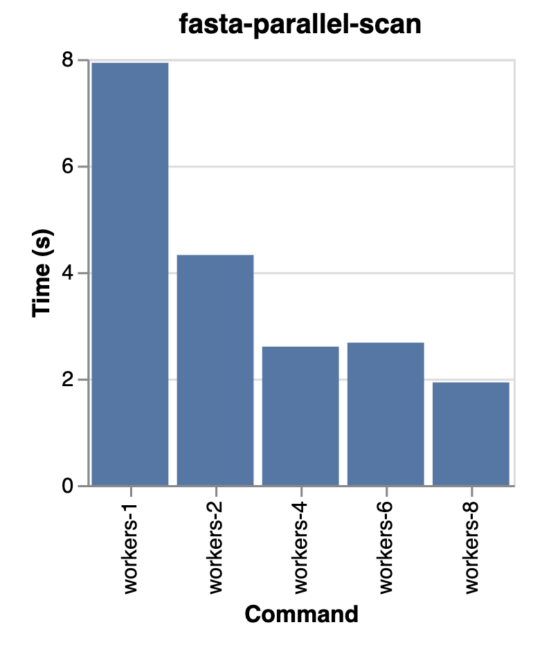
And Exon will distribute reading the files across available cores. This is a huge win for data lakes, where you can now read multiple files in parallel without having to manually shard your data. E.g. here we see a 4x speed-up when reading 8 files.

MzML Reader​

MzML is a very common format in metabolomics and proteomics. At its core are measurements of the spectrum from the mass spec, but there's also a Controlled Vocabulary that describes various metadata about the experiment.

Similar to other readers, you instantiate a reader and then depending on what you want to do with it, you can convert it to arrow or polars with BioBear, or a data.frame with R.

import biobear as bb

# object stores and local files are supported
df = bb.MzMLReader("mzml-data/GNPS00002_A3_p.mzML").to_polars()

df.head()
# shape: (5, 6)
# ┌───────────────────────────────────┬───────────────────────────────────┬───────────────────────────────────┬────────────┬───────────────────────────────────┬────────────────┐
# │ id                                ┆ mz                                ┆ intensity                         ┆ wavelength ┆ cv_params                         ┆ precursor_list │
# │ ---                               ┆ ---                               ┆ ---                               ┆ ---        ┆ ---                               ┆ ---            │
# │ str                               ┆ struct[1]                         ┆ struct[1]                         ┆ f32        ┆ object                            ┆ object         │
# ╞═══════════════════════════════════╪═══════════════════════════════════╪═══════════════════════════════════╪════════════╪═══════════════════════════════════╪════════════════╡
# │ controllerType=0 controllerNumbe… ┆ {[80.948143, 80.993134, … 957.16… ┆ {[5416.88916, 7712.663574, … 480… ┆ null       ┆ [('MS:1000579', {'accession': 'M… ┆ None           │
# │ controllerType=0 controllerNumbe… ┆ {[80.284782, 81.017242, … 1176.3… ┆ {[4701.711426, 5527.709961, … 95… ┆ null       ┆ [('MS:1000579', {'accession': 'M… ┆ None           │
# │ controllerType=0 controllerNumbe… ┆ {[80.948288, 81.017365, … 1193.9… ┆ {[11152.501953, 9900.050781, … 8… ┆ null       ┆ [('MS:1000579', {'accession': 'M… ┆ None           │
# │ controllerType=0 controllerNumbe… ┆ {[80.948143, 81.017372, … 1074.1… ┆ {[6677.85791, 11401.181641, … 12… ┆ null       ┆ [('MS:1000579', {'accession': 'M… ┆ None           │
# │ controllerType=0 controllerNumbe… ┆ {[80.948174, 81.017387, … 968.84… ┆ {[6586.833984, 13542.833008, … 6… ┆ null       ┆ [('MS:1000579', {'accession': 'M… ┆ None           │
# └───────────────────────────────────┴───────────────────────────────────┴───────────────────────────────────┴────────────┴───────────────────────────────────┴────────────────┘

For R users, see the read_mzml_file function. And for exon-duckdb users see

Please see the docs for more information about MzML files, and again, please let us know if you have any feedback!

A Sneak Peak for Querying​

While it's not quite ready yet for BioBear and ExonR, in Exon, we've added a set of MzML specific functions for querying. For example, you can filter spectra based on the presence of a specific peaks.

For example, this will filter a set of spectra to only those that have a peak at 100.0 m/z that's within 0.1 m/z of the peak.

SELECT id
FROM mzml -- same table as above
WHERE contains_peak(mz.mz, 100.0, 0.1) = true

This sort of declarative informatics is part of the Exon vision, which we'll be talking more about in the future.

A Note on Performance​

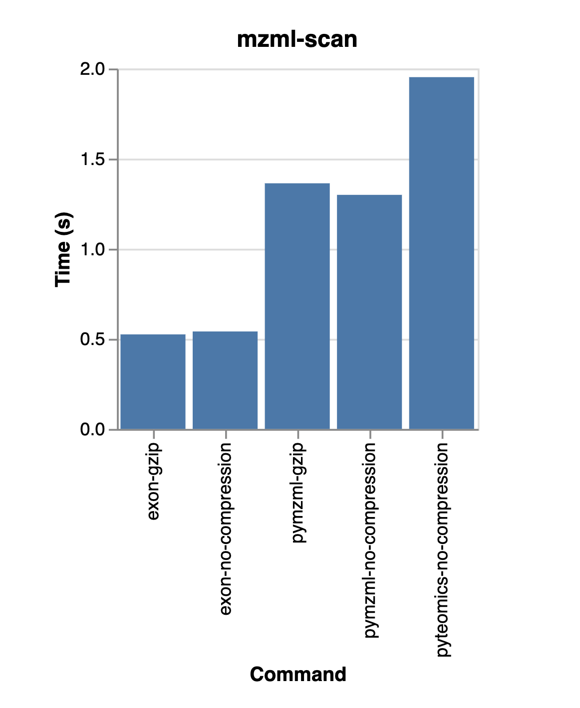
Similar to BioBear comparing favorably to other scientific data libraries, we see modest out-performance for MzML file reading.

The following compares reading using a few difference libraries in Python on an MzML file with about 8k spectra.

Pandas Support in BioBear​

There's not much to say besides that places where you could use to_polars you can now also use to_pandas. E.g.

import biobear as bb
from pathlib import Path

data = Path("./data/uniref50.fasta")
df = FastaReader(data).to_pandas()  # need to install pandas

df.head()
#                     id                                        description                                           sequence
# 0  UniRef50_A0A5A9P0L4  peptidylprolyl isomerase n=1 Tax=Triplophysa t...  MEEITQIKKRLSQTVRLEGKEDLLSKKDSITNLKTEEHVSVKKMVI...
# 1  UniRef50_A0A410P257  Glycogen synthase n=2 Tax=Candidatus Velamenic...  MKAIAWLIVLTFLPEQVAWAVDYNLRGALHGAVAPLVSAATVATDG...
# 2  UniRef50_A0A8J3NBY6  Gln_amidase domain-containing protein n=2 Tax=...  MEILGRNLPRILGNLVKTIKTAPVRVVARRGARTLTQKEFGKYLGS...
# 3      UniRef50_Q8WZ42  Titin n=3053 Tax=cellular organisms TaxID=1315...  MTTQAPTFTQPLQSVVVLEGSTATFEAHISGFPVPEVSWFRDGQVI...
# 4  UniRef50_A0A401TRQ8  Ig-like domain-containing protein (Fragment) n...  PPSFIHKPDPQEVLPGSNVKFTSVVTGTAPLKVSWFKGTTELVAGR...

Conclusion​

We hope you enjoy the new features and please let us know if you have any feedback! We'll be back next month with more updates.

Conda has become a popular way to distribute software in the bioinformatics community. We're excited to announce that we've added BioBear to Conda Forge. You can now install BioBear with the following command:

conda install -c conda-forge biobear

Pip still works as well:

pip install biobear

We're excited release ExonR. This is an R package that allows for interacting with Exon through an ergonomic R interface.

Usage​

As a quick example, we can read in a GFF file from S3 and convert it to a GRanges object.

library(exonr)
library(GenomicRanges)

rdr <- read_gff_file(
  "s3://bucket/path/to/file.gff",
)

df <- as.data.frame(rdr)

gr <- GRanges(
  seqnames = df$seqname,
  ranges = IRanges(
    start = df$start,
    end = df$end,
  ),
)

Installation​

If you're on an x64 machine, you should be able to install a pre-built binary from our R-universe.

install.packages('exonr', repos = c('https://wheretrue.r-universe.dev', 'https://cloud.r-project.org'))

This should also build on other platforms, but you'll need to have Rust installed. The main Rust website has a guide for installing rust. Once you have rust installed, you can install ExonR from source with the command above.

• Exon
  • Demonstration
• BioBear
• Object Stores
• Better Home and Docs Site
• Open Source

It's been around six weeks since our last public update. Here's what we've done:

1. We've refactored our DuckDB extension into a standalone Rust library named Exon. This is a Rust-based library designed to implement a SQL engine that's aware of scientific data types and workflows.
2. The DuckDB extension now utilizes Exon and has been renamed as Exon-DuckDB. This can be used with Python, R, and C++, wherever DuckDB is used.
3. We've also released an open-source Python package, BioBear, which connects Exon with PyArrow and Polars.
4. Exon, along with its DuckDB extension and BioBear, now supports Object Stores such as S3 and GCS. Local paths like ./path/to/file can be replaced with cloud storage paths like s3://bucket/path/to/file or gs://bucket/path/to/file, and the code will function the same.
5. We've set up a documentation site with additional examples and tutorials, including Delta Lake integration and neighborhood analysis, similar to a map that helps users navigate.
6. Finally, the libraries have been made open-source under permissive licenses. We hope that this will prompt others to use and contribute to the project, aiding in the development of a community around these tools.

Exon​

Exon is a library written in Rust that takes advantage of DataFusion to develop a SQL engine proficient in handling scientific data types and workflows. It's designed for embedding into other applications and is the cornerstone of our DuckDB extension and BioBear packages.

This core infrastructure allows easy data management via Arrow and/or SQL and ensures adaptability across different execution environments. BioBear is specifically a Python package, but the Exon-DuckDB extension is adaptable, operating wherever DuckDB is used, such as Python, R, and JavaScript. We're currently exploring other language bindings, so feel free to reach out if you'd like to see a specific language supported.

See the Exon documentation, which has links to the installable crate, the Rust docs, and more.

Demonstration​

For a brief demonstration, let's examine how we can use Exon to scan a GFF file, an output of CRT from a JGI dataset, and join the CRISPR array annotations with repeat units entirely within the array. If Rust isn't your focus and you're primarily interested in utilizing this code as a library, move forward to the BioBear section.

use arrow::util::pretty::pretty_format_batches;
use datafusion::error::DataFusionError;
use datafusion::prelude::*;
use exon::context::ExonSessionExt;

#[tokio::main]
async fn main() -> Result<(), DataFusionError> {
    let ctx = SessionContext::new_exon();

    let path = "./exon-examples/data/Ga0604745_crt.gff";
    let sql = format!(
        "CREATE EXTERNAL TABLE gff STORED AS GFF LOCATION '{}';",
        path
    );

    ctx.sql(&sql).await?;

    let df = ctx
        .sql(
            r#"SELECT crispr.seqname, crispr.start, crispr.end, repeat.start, repeat.end
            FROM (SELECT * FROM gff WHERE type = 'CRISPR') AS crispr
                JOIN (SELECT * FROM gff WHERE type = 'repeat_unit') AS repeat
                    ON crispr.seqname = repeat.seqname
                    AND crispr.start <= repeat.start
                    AND crispr.end >= repeat.end

            ORDER BY crispr.seqname, crispr.start, crispr.end, repeat.start, repeat.end
            LIMIT 10"#,
        )
        .await?;

    // Show the logical plan.
    let logical_plan = df.logical_plan();
    assert_eq!(
        format!("\n{:?}", logical_plan),
        r#"
Limit: skip=0, fetch=10
  Sort: crispr.seqname ASC NULLS LAST, crispr.start ASC NULLS LAST, crispr.end ASC NULLS LAST, repeat.start ASC NULLS LAST, repeat.end ASC NULLS LAST
    Projection: crispr.seqname, crispr.start, crispr.end, repeat.start, repeat.end
      Inner Join:  Filter: crispr.seqname = repeat.seqname AND crispr.start <= repeat.start AND crispr.end >= repeat.end
        SubqueryAlias: crispr
          Projection: gff.seqname, gff.source, gff.type, gff.start, gff.end, gff.score, gff.strand, gff.phase, gff.attributes
            Filter: gff.type = Utf8("CRISPR")
              TableScan: gff
        SubqueryAlias: repeat
          Projection: gff.seqname, gff.source, gff.type, gff.start, gff.end, gff.score, gff.strand, gff.phase, gff.attributes
            Filter: gff.type = Utf8("repeat_unit")
              TableScan: gff"#,
    );

    // Uncomment to show the physical plan, though it's obviously messier.
    // let physical_plan = df.create_physical_plan().await?;
    // println!("Physical plan: {:?}", physical_plan);

    // Collect the results as a vector of Arrow RecordBatches.
    let results = df.collect().await?;
    let formatted_results = pretty_format_batches(results.as_slice())?;
    assert_eq!(
        format!("\n{}", formatted_results),
        r#"
+------------------+-------+------+-------+-----+
| seqname            | start | end  | start | end |
+------------------+-------+------+-------+-----+
| Ga0604745_000026 | 1     | 3473 | 1     | 37  |
| Ga0604745_000026 | 1     | 3473 | 73    | 109 |
| Ga0604745_000026 | 1     | 3473 | 147   | 183 |
| Ga0604745_000026 | 1     | 3473 | 219   | 255 |
| Ga0604745_000026 | 1     | 3473 | 291   | 327 |
| Ga0604745_000026 | 1     | 3473 | 365   | 401 |
| Ga0604745_000026 | 1     | 3473 | 437   | 473 |
| Ga0604745_000026 | 1     | 3473 | 510   | 546 |
| Ga0604745_000026 | 1     | 3473 | 582   | 618 |
| Ga0604745_000026 | 1     | 3473 | 654   | 690 |
+------------------+-------+------+-------+-----+"#
    );

    Ok(())
}

BioBear​

BioBear is a Python package that extends Exon, providing it with a Pythonic interface. For instance, you can read a GFF file from S3, and then load it into a PyArrow RecordBatch Reader and/or a Polars DataFrame.

PyArrow's strength lies in its ability to render our domain-specific data highly portable. For instance, suppose you have a Python job that produces a GFF file, perhaps the output of Prodigal. You can create an Arrow RecordBatch Reader that streams data from S3 into a Delta Lake table.

import biobear as bb
from deltalake import write_deltalake

batch_reader = bb.GFFReader("./job/output/test.gff").to_arrow()

write_deltalake("s3a://bucket/delta/gff", batch_reader, storage_options={"AWS_S3_ALLOW_UNSAFE_RENAME": 'true'})
# aws s3 ls s3://bucket/delta/gff
#                            PRE _delta_log/
# 2023-06-24 11:00:19    8509556 0-ccedd844-373f-4e70-a99e-2167535fcf35-0.parquet

You can also use BioBear to query local indexed files. For example, you can query a BCF file for records on chromosome 1.

import biobear as bb

reader = bb.BCFIndexedReader("example.bcf")
df = reader.query("1")

In this case, the query is executed by the BCFIndexedReader, which uses the index to only read the records on chromosome 1. This is much faster than reading the entire file and filtering in memory.

Object Stores​

Scientific computing is increasingly done in the cloud -- the data that gets generated from workflows is plopped somewhere in you favorite object store (e.g. S3). This has made it less expensive to store the output but adds an additional layer of complexity when trying to do analysis.

To try to mitigate this complexity WHERE TRUE's tools now support reading from object stores. For example, we could rewrite the last example to read from S3:

import biobear as bb
from deltalake import write_deltalake

batch_reader = bb.GFFReader("s3://bucket/job/output/test.gff").to_arrow()
write_deltalake("s3a://bucket/delta/gff", batch_reader, storage_options={"AWS_S3_ALLOW_UNSAFE_RENAME": 'true'})

Put this in a lambda and you're about 3/4ths of the way to a cloud-based bioinformatics data platform.

Or, if DuckDB is more your speed, you can do:

SELECT *
FROM read_gff('s3://bucket/job/output/test.gff')

Better Home and Docs Site​

We'll, you're here aren't you... kidding of course, but we've deployed an update to the main site and the docs site. The docs have more examples. We gave the example earlier of how to use BioBear to write a Delta Lake table from a GFF file. We also have an example of how to use Exon-DuckDB to do neighborhood analysis on a metagenomics sample.

Have a gander at our main site here.

Open Source​

The ultimate goal of WHERE TRUE Technologies is to not exist. We want to build tools and popularize techniques that diminish the need for the majority of specialized bioinformatics file formats in favor of more general-purpose formats that are easier to work with, but don't make tradeoffs on performance or flexibility.

To get to that state, we've opened sourced our libraries under permissive licenses. We hope that this will encourage others to adopt and contribute to the project, and help us build a community around these tools.

You can review the licenses for each of the libraries at the following links:

• Exon
• BioBear
• Exon-DuckDB